Processing Notes

Location: Riet Vell

Author: Angèlica Busquets Rubiés

Date: 2025-09-08

Processed period: 2025-01-01 (01) to 2025-09-04 (247)

Code: L0, L1, L2, L3

 

Flux processing L0

We lost flux data from 11^th to 14^th of May (131-134), from 3^rd to 8^th of July (184-189), and from August 16^th until 4^th of September (228-247). So there are no files for these days.

In DOYs 1-9, 13-29,37, 155-164, CH4 concentrations are NaN due to null RSSI. This is probably because of the sensor’s desynchronization, that got ‘fixed’ every time we went to the field (see example doy 8).

In doy 38, the data starts after midday because it is the moment we switched sensors from 10Hz to 20Hz.

 

 

Some days have a RSSI periodic pattern. It is prob. due to the self-cleaning system (see example doy 63).

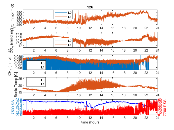
From doy 119 until the end, there are many days where RSSI is highly variable, so CH4 concentrations have a lot of filtered data (example of doy 126). It is when spiderwebs started appearing, so it could be that with the wind the spiderwebs interfere with the sensor.

In doys 173-176 and 177-183 (on 184 flux data stopped recording), LI7500 has very low SS, and no filtered concentration data. We went to the field the 176 and on 190. This matches with the fact that the Li7500 had a nest right under the top lens both times we went to clean it.

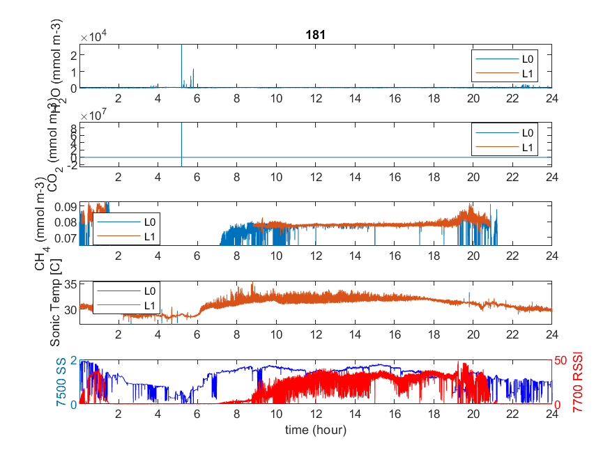
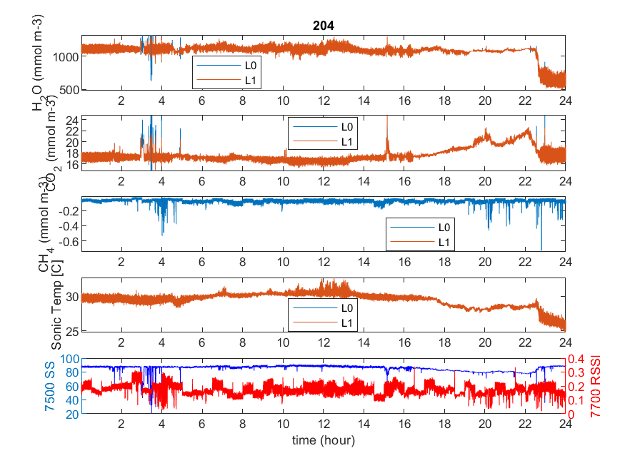
From 201 to 205, RSSI is too low and Li7700 does not have any filtered CH4 concentration.

 

 

Flux processing L1/L2

 

Lags: Using the GetLag function and CalculateLags script, I have checked the points that W lags Q and later got the lag in seconds. I have found different lags for the period where the frequency was 10Hz and for the one that it was 20 Hz:

• For 10Hz, the maximum lag is 654 points = 65,4s. So, for ‘lag_cq_range’ I put +-70s.
• There were no lags found in 20Hz data. Max of 2 points (0.1s). So, for ‘lag_cq_range’ I put +-0.3s.

Period 1

Period 2

 

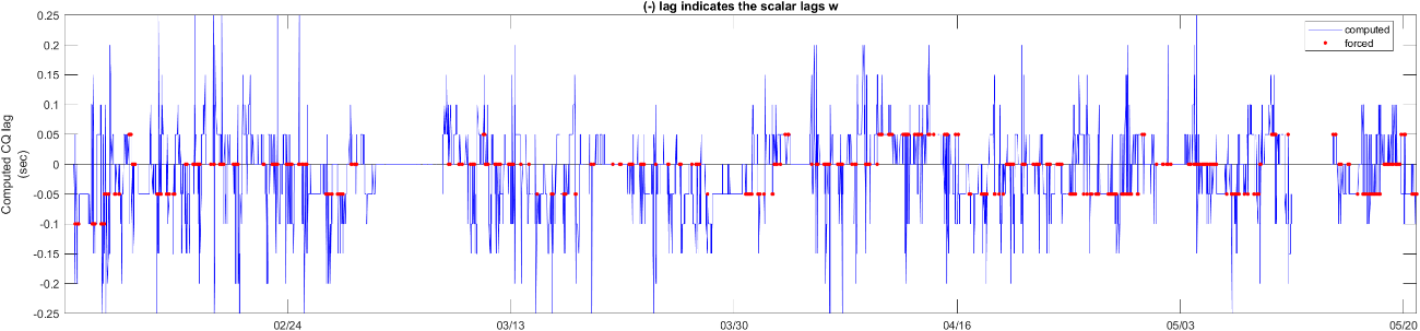
L1L2 data is processed in 3 periods:

• 1^st period: From DOY 001 to 037, where frequency was 10Hz, there was a lag of 65.4s (+-70) and z_veg was 0.
• 2^nd period: From 038 to 140, where frequency was 20Hz, there was no lag (+-0.3) and z_veg was 0. We also checked with 10s to see if the results were similar, and they were.
• 3^rd period: From 141 until 228 (note July 2026: I re-run these periods because there was a mistake with the calculated ze for gaps. In the end, for this period I added until 247, to be able to include the gap of august), where frequency was 20Hz, there was no lag (+-0.3) and z_veg was 78 cm– at doy 141 (21^st of may) the field was flooded and plants started getting higher. 78cm is the mean of the measured vegetation heights in July, august and september + an approximation of the height in May and June where no measurements were taken (40cm in May, 60 cm in June, 82 cm in 09/07, 90.5 cm in 24/07, 97.2 cm in 05/08, 100.7 cm in 04/09).

 

1st period

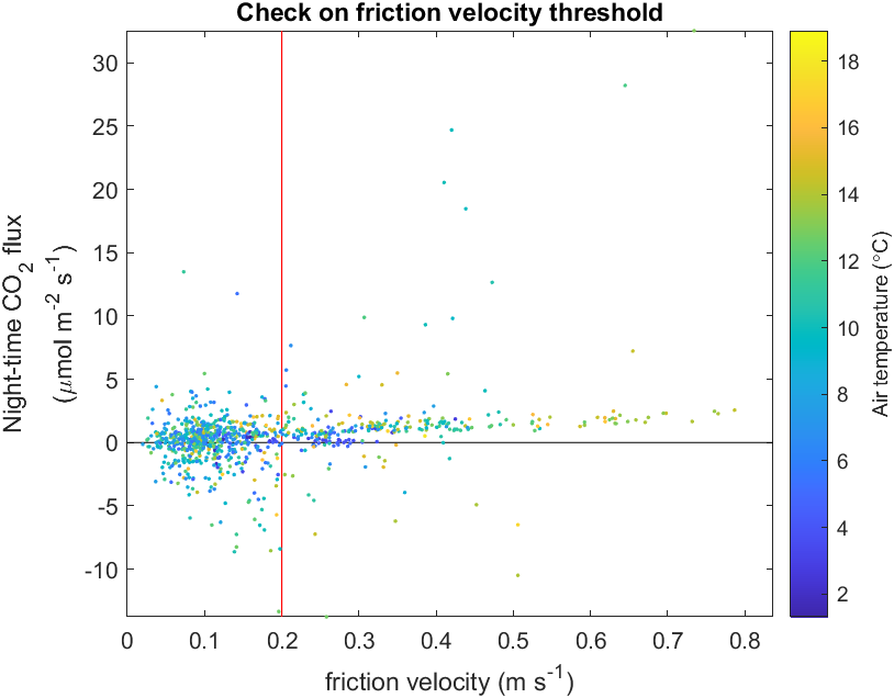
The results I got for the 1^st period are very suspicious. To begin with, there are a lot of negative CO2 fluxes. I have set a filter of 0.2m/s. However, this is very strict and filters a lot of data.

The flux patterns are also weird. There is a daily cycle in heat fluxes, but LE is sometimes very high when H is very negative.

Carbon fluxes do not follow a clear pattern. That could be because almost no vegetation was at the field in that period. As we already knew from L0, there are large CH4 flux gaps.

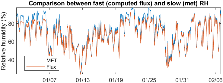
When comparing met and flux RH and T values, some differences can be seen. Met RH achieves higher values than RH Flux values. And for Temperature there seems to be a bit of lag between Met T and Flux T. In addition, Met T achieves lower values than Flux T.

The Energy Balance Closure is extremely low, indicating a poor energy flux balance.

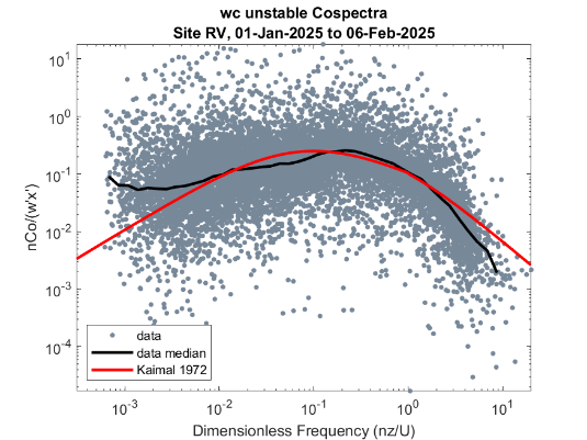
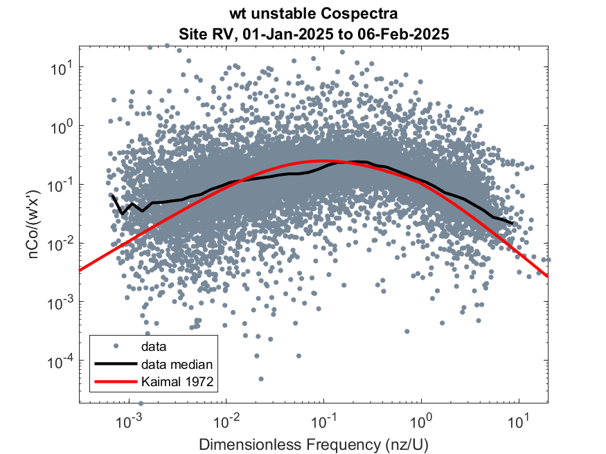
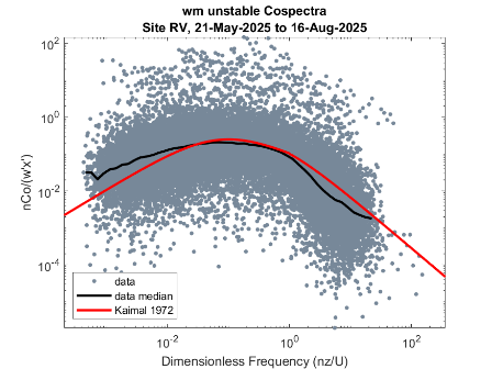
For the cospectra, lower frequencies seem to be overestimated, and higher frequencies underestimated (except for wt).

 

 

When computing the footprint for this period, the results are very large. A footprint of this scale is very unusual for this type of site.

 

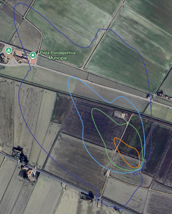
For this reason, we decided to leave this period out for the moment, until we understand better the results. Maybe the configuration of the tower software was wrong, and we fixed it when we changed from 10 to 20 Hz.

 

2n period:

This period’s results are more reasonable.

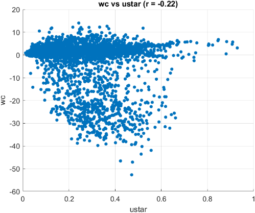
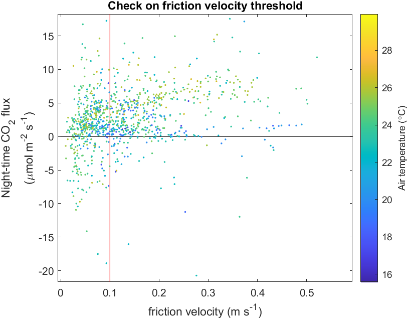
I did not add any ustar threshold, since there is not a clear relationship between negative nighttime co2 flux and friction velocity.

 

Heat fluxes follow a clear daily pattern, with LE exciding H until beginning of April. Our field was only flooded until around February, but the contiguous field was flooded until later (check footprint, which reveals high influence from this other field. Still, most data comes from our field, check later computations with wind filter). However, I find the end of April to be very late for having such high LE with a drying soil. Maybe there is advection of moist air from the sea, or dew (difficult at this time of the year…). Similarly to period 1, but less frequently, there are moments when H is minimum and very negative and LE is maximum. Maybe it happens at sunrise hours, with a moist field, when there is an increase in the evaporation and it cools down the soil? Check hours when it happens -> during night hours. Datestr( ) can be used to convert Mdatetime to readable datetime format. If the plot ticks do not have decimals and the hour cannot be known, create a data tip and right-click on it -> Edit content and style. You’ll see a popover that has “DataTipRows”. Click that and then click the field you want to adjust. Format is set to AUTO. Type in the precision you want into that field using MATLAB’s standard nomenclature, so for 9 spaces and 3 decimal points as a float: %9.3f   .

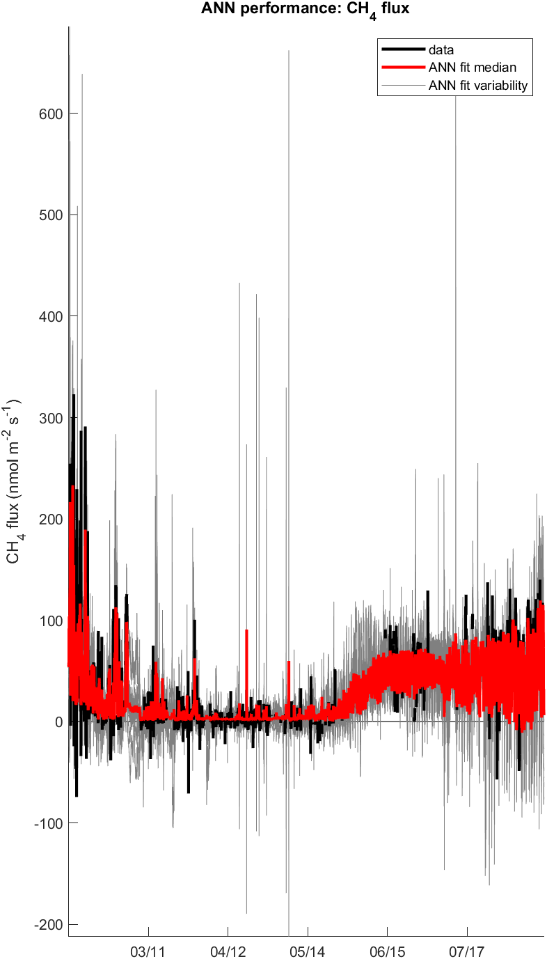
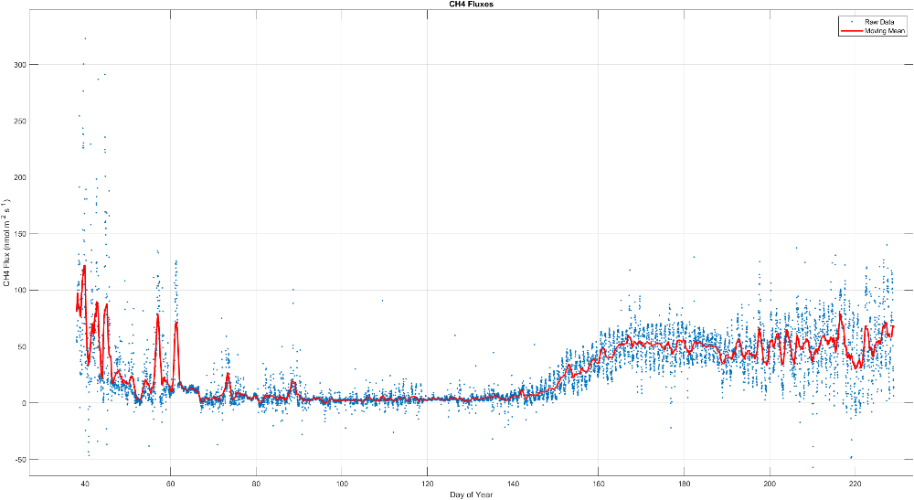
CO2 fluxes do not show clear patterns since almost no vegetation had grown at the field yet. CH4 fluxes reveal higher emissions during January and February, probably due to the fields still being flooded.

 

For HR and T, met and flux values still show a similar behavior as period 1. Met HR is higher than Flux HR (reaching a 20% difference). And T seems a bit lagged at decreasing as well as Met T consistently reaching lower values than Sonic T periods (as if sonic T took longer time to ‘cool off’).

 

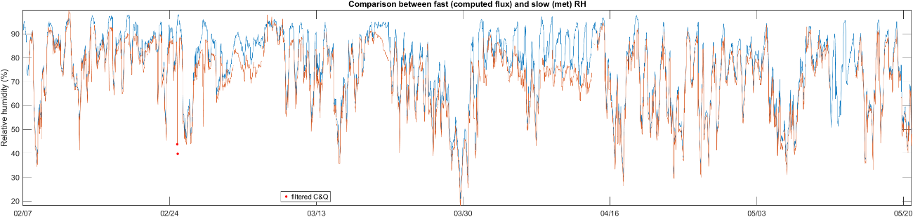
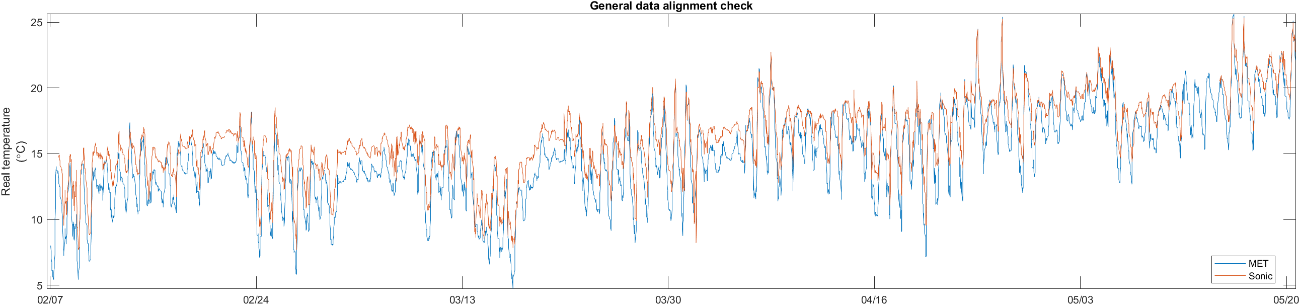
In this period, the EBC is more aligned with what we would expect.

 

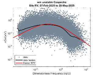
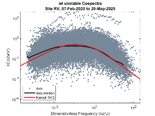
Cospectra follows a similar pattern to Period 1:

 

Footprint reveals high influence from the field nearby. For this reason, and considering that this other field has different elevation and water levels, we decided to make another series of data with the contributions of the NE field filtered.

 

3rd period

I set a ustar filter of 0.1 m/s. 

 

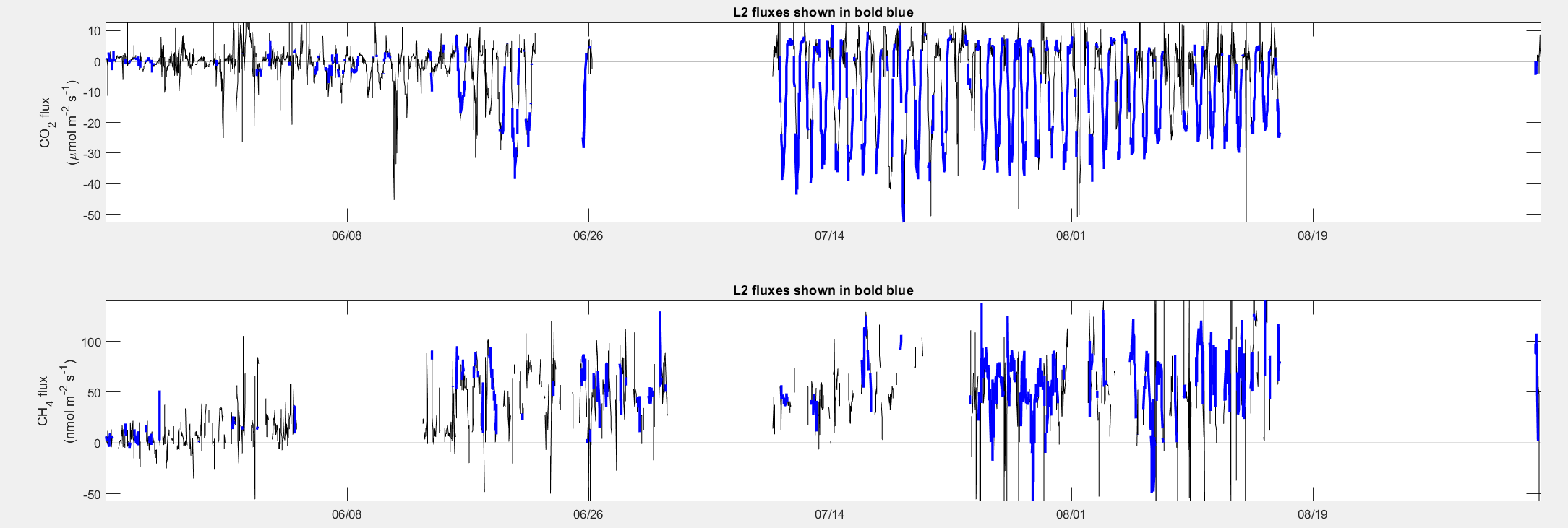
During June and July, many flux series have gaps because of the low SS and RSSI (spiderwebs and nests) and because of the sudden stop of flux data recording.

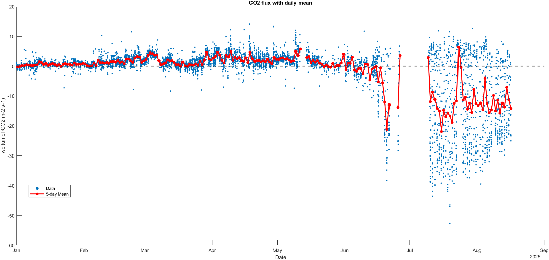
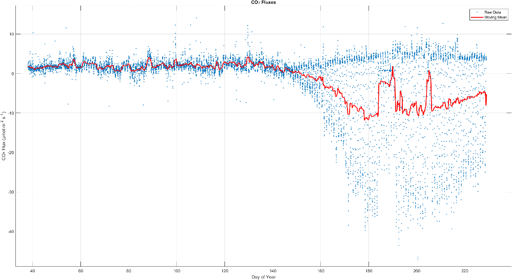
LE dominated over H during the whole period. CH4 series reveals higher emissions as the months go by. CO2 fluxes reveal a clear daily pattern from at least July, with a clear uptake during the day and a bit of emission during the night.

 

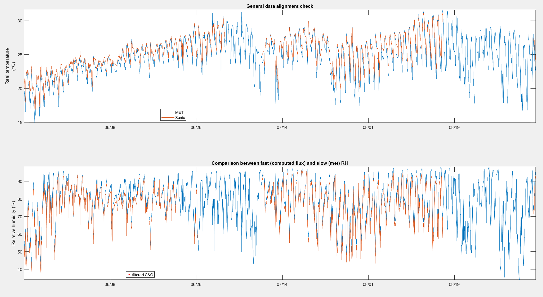
For RH and T comparison between Met and Flux values, they are much better aligned with each other than previous periods but still have some lag and amplitude differences.

 

 

 

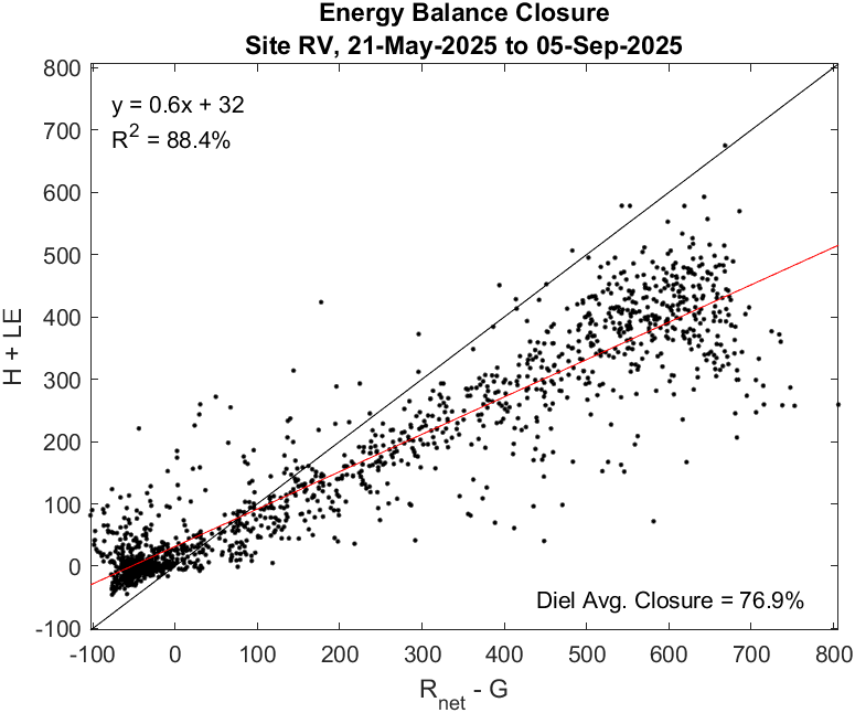
The EBC is also as expected. It is a low closure (60%), but typical for wetlands.

 

Cospectra shows similar pattern as previous periods. 

 

 

 

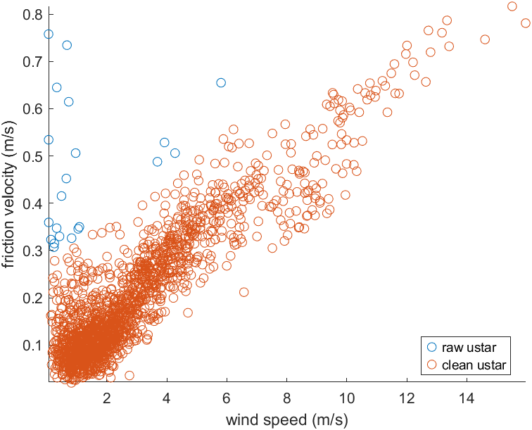
P1 and P3, respectively. When checking correlation between wind speed and friction velocity, we see that P3 has 2 different linear correlations.

 

 

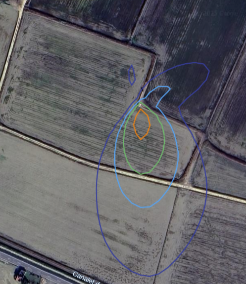
The footprint shows a main contribution from south upwind area.

 

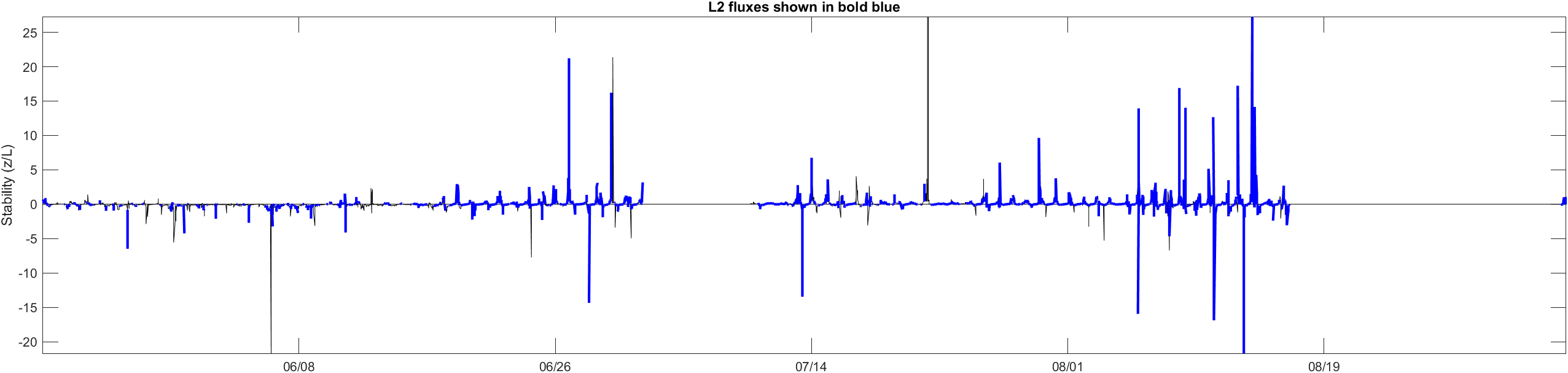
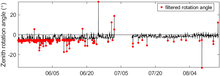
All periods also showed a high zenith rotation angle. From July until August the filtered zenith rotation angles decrease a lot. 2nd of October we went to the field and corrected the slight inclination by putting the anemometer as straight as we could. We should revise if this corrects the rotation angle (the mean should be closer to 0).

 

The whole carbon fluxes series with its 5-day mean is represented below:

  

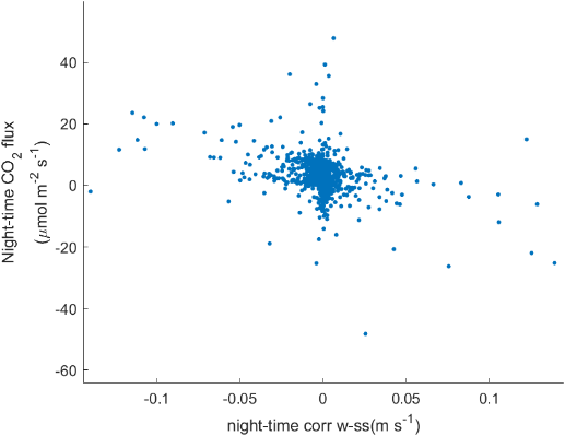
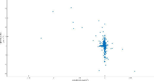
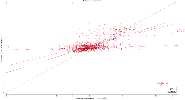
In Period 1, nighttime w’ss’ and nighttime CO2 fluxes have no correlation, meaning that the negative nighttime CO2 fluxes observed in the ustar plot do not come from an artefact of SS. The result is very similar for P2. For Period 3 there seems to be a negative correlation between the two variables, but only with a few data points, while the bast majority of negative nighttime CO2 fluxes are not correlated with w’SS’.

 

P1                                                                        P3

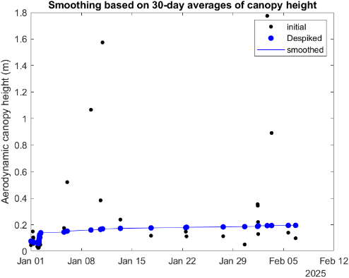
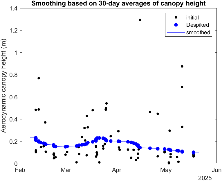
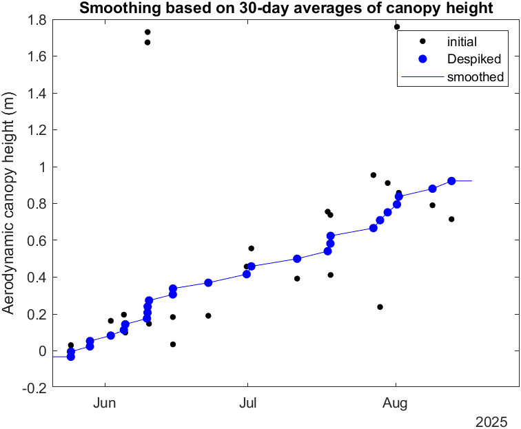
For some reason that I have not been able to comprehend, I rerun the code and obtained different results for aerodynamic canopy plots. It looks like the first time not all data was being used. This happened with all periods, but only for the canopy plots. I did not make any changes to the code neither to the input files, and github shows no changes either.

The different graphs are:

P1:

 

P2:

 

P3: it reflects the growing of the rice

Revising the aerodynamic canopy height function called …., we realitzed that we needed to add the wind filter. I also changed one nanmean to mean and omitnan. I rerun the wind filtered L1L2 with the actualized

This did not change the results

 

 

Wind direction filter

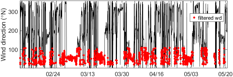
Now, I rerun the L1L2 code but filtering out the wind directions from 20º to 110º (the contiguous field).

 

P2:

Diel average ebc improved a bit up to 90.5%.

Weirdly, aerodynamic canopy height plot is the same I got the first time (the one with less data points). I do not understand why this happens.  And now I rerun it without wind filters and get again less points…

More fluxes than before are filtered, but the majority is still from desired angles.

 

P3:

Canopy aerodynamic height is the same as the one with less dots.

Ebc remains similar.

The period from May to June gets very filtered for the wind condition.

 

 

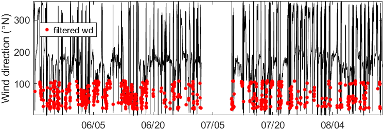
P1:

Did not include in the combine.

Ebc still very bad.

Some fluxes are filtered out, but not so many.

 

 

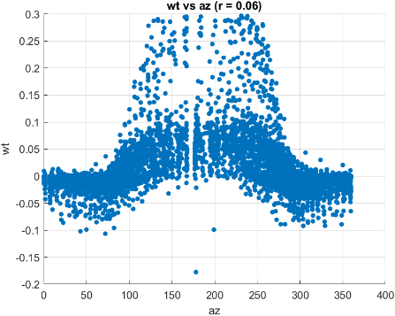
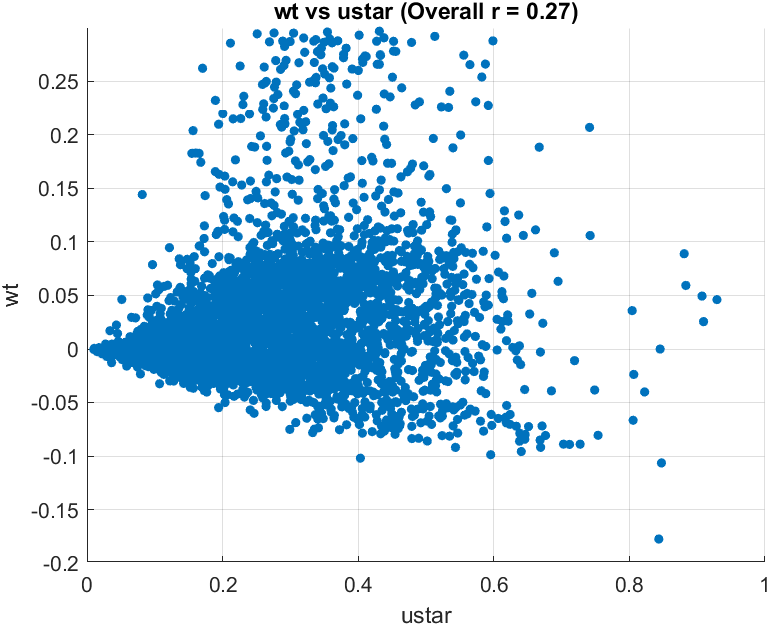
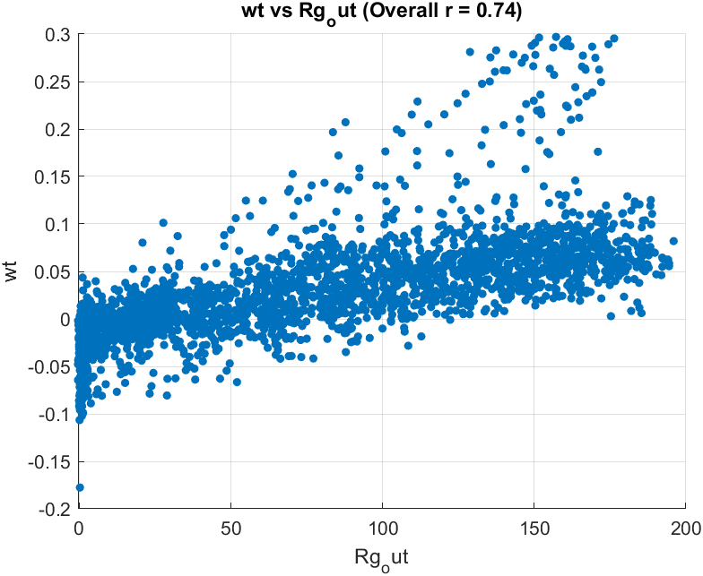
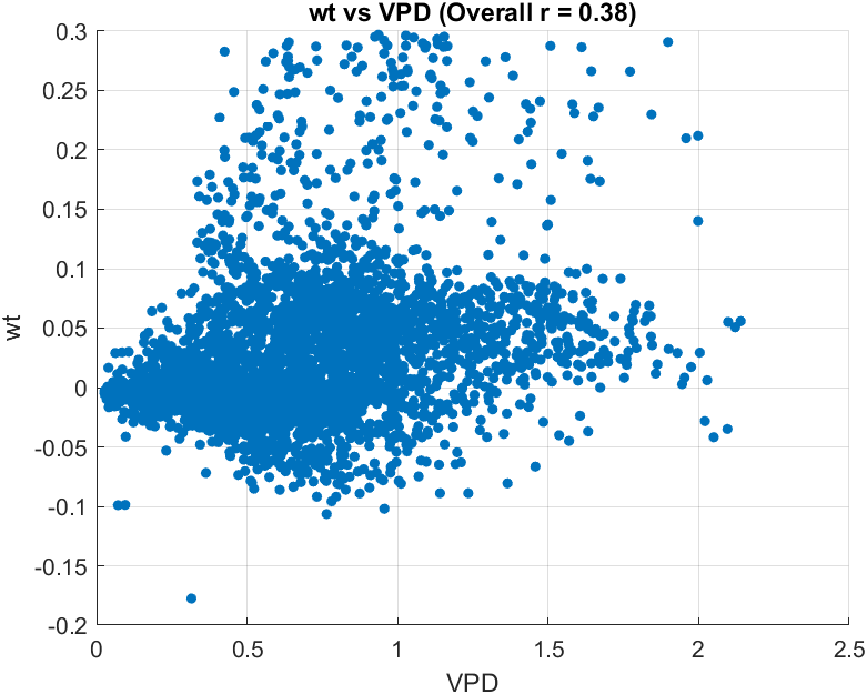
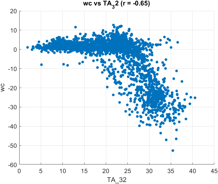
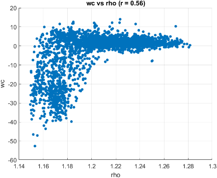
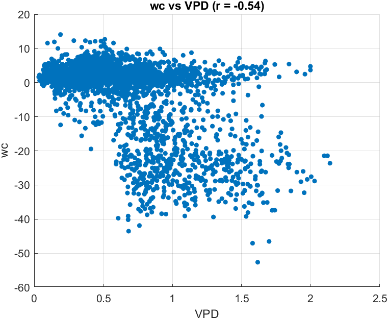
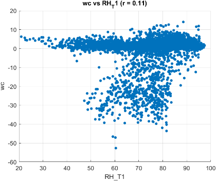
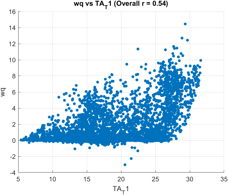
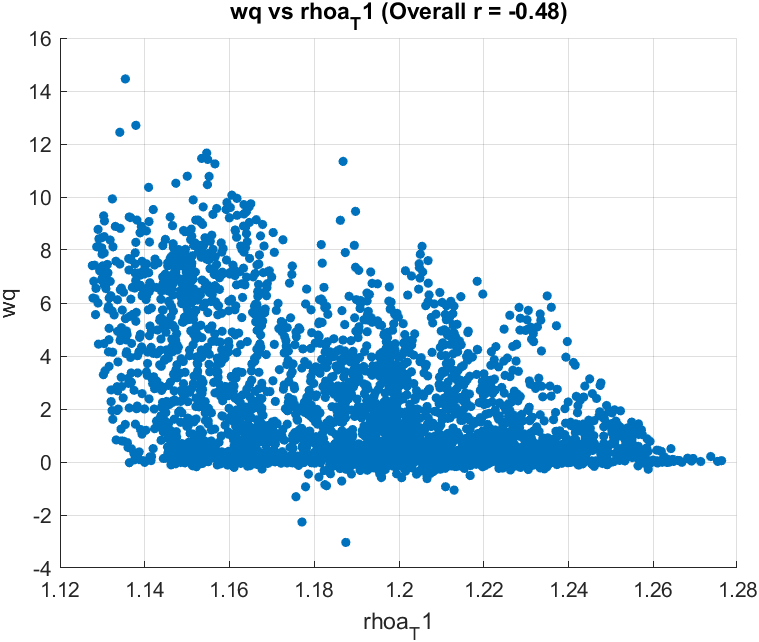
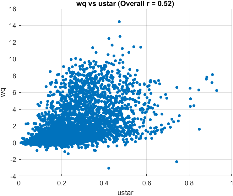
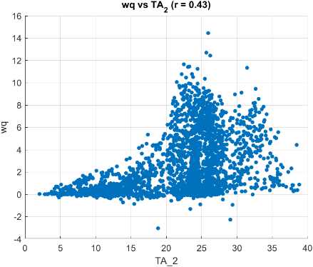
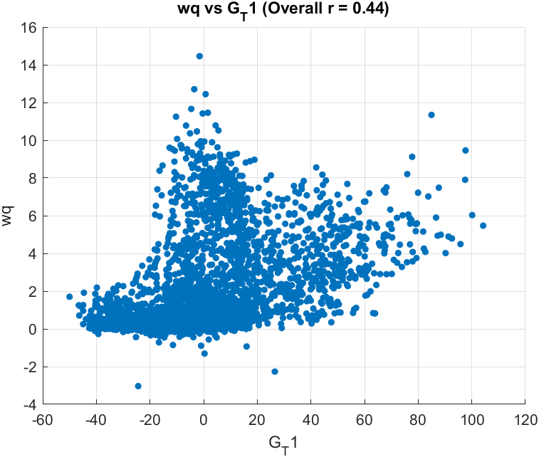
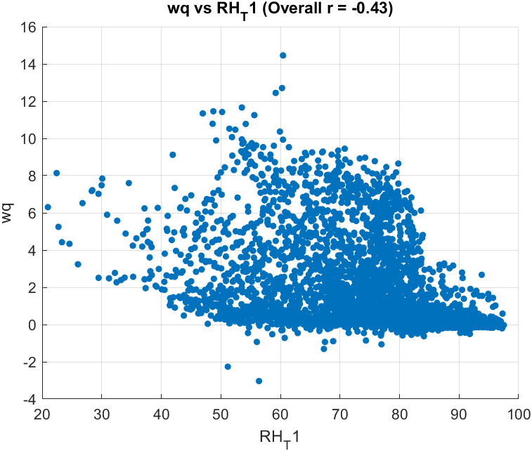
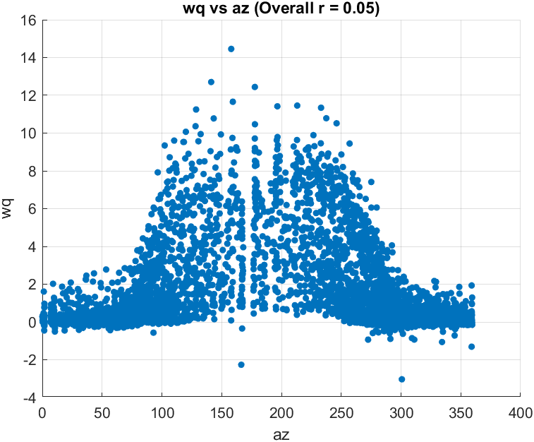
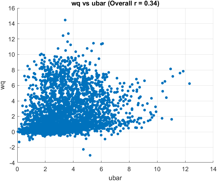
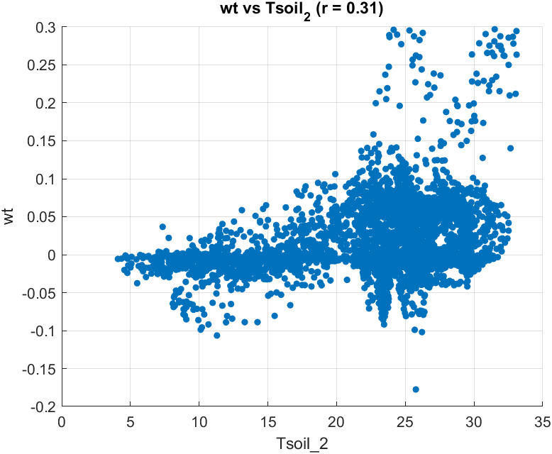
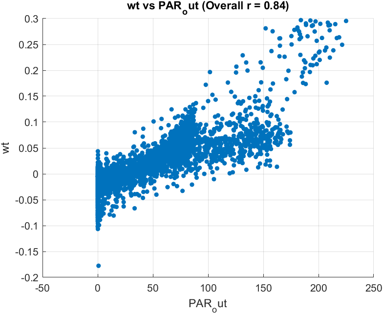
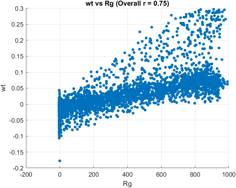
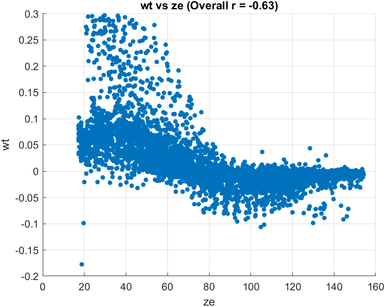
(pictures of variable correlations shown in the end of the text)

L3

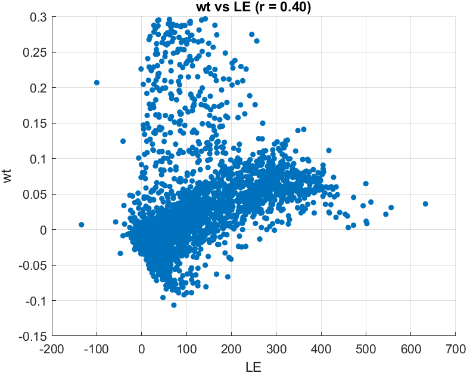
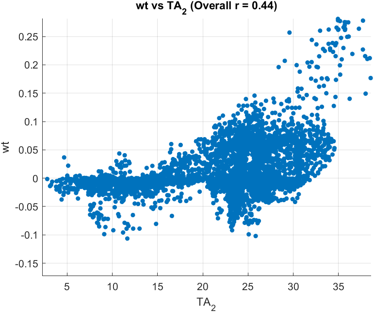
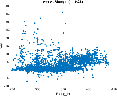
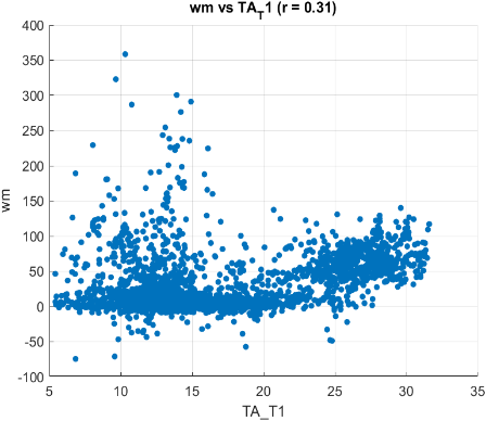
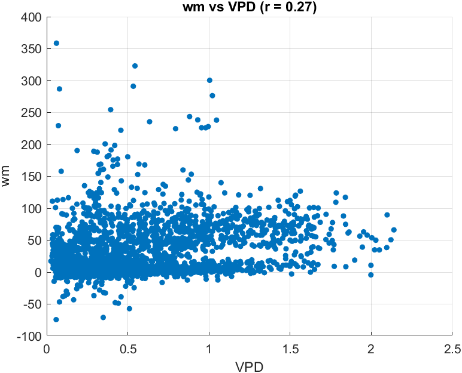
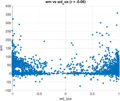
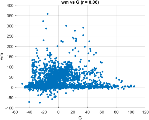
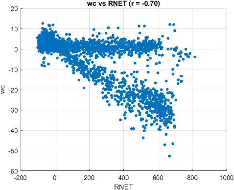
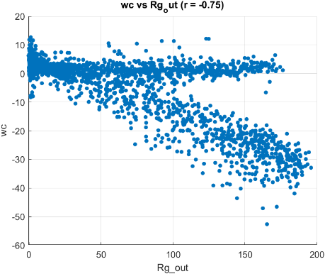
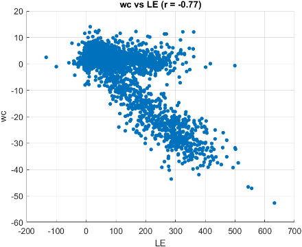
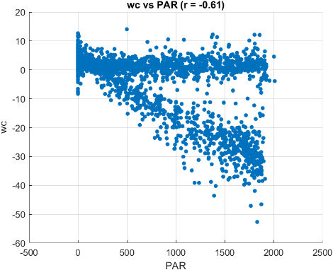
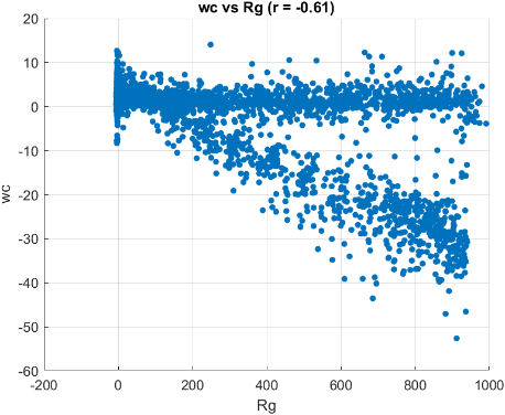
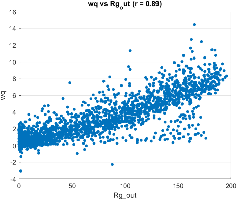
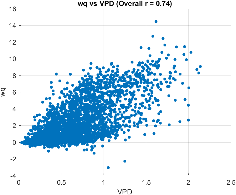
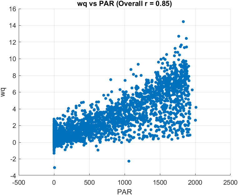
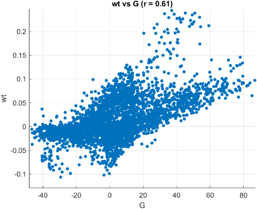
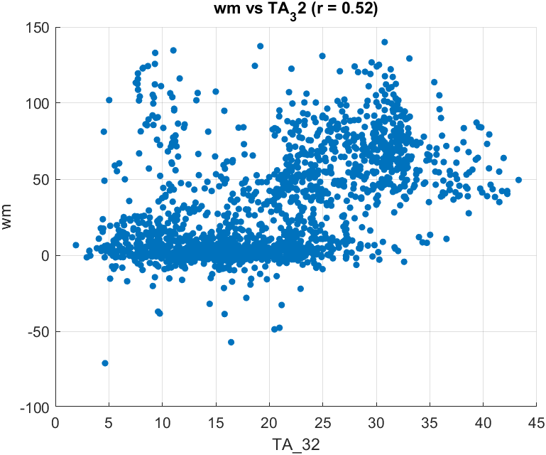
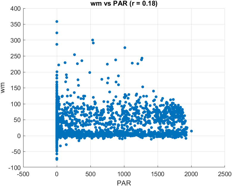
I use the script L3_corr (located in …eddycovariancegeneral\CentralizedFluxCode\Extras) to check for variables that can have a strong correlation with flux variables, to decide which ones we can use for the gap filling process. This code creates a dataset combining metdata with fluxdata, since L2 does not have all met variables.

The graphs show the variables which have some kind of correlation. Some of them are omitted if they are redundant (i.e., TA_2 and TA_4 show very similar results, I only show the one with higher correlation).

I also annotate the variables I decide to use for the L3 gap filling, considering higher correlations and lower gaps, as well as the opts file of other sites.

Some of the plots show two very different behaviors. Although day/night plays a role, there is a very high influence of season with and without vegetation. I think in the future we should address this.

wt: RNET, ze, az, TA_32cm (TA has very low corr), VPD, WD_cos (would it be better to use ustar instead of VPD or WD_cos? And WD_sin instead of WD_cos?),

Wq: TA (TA_32 has higher corr, but has more gaps), RNET, ze, az_cos, VPD, ustar (should we add tsoil_2? We could subst for one of the angles)

Wc: PAR, TA, VPD, az, ustar (dec-day_since_mow)

Wc GPP/ER partitioning: TA, ustar, par

Wm: WD_cos, TA, rlong_in, vpd, ustar, LE_gf?->LE_ngf (in the other sites: gpp and er ann night?)

 

Results after gap filling:

  

 

 

 

 

 

 

 

 

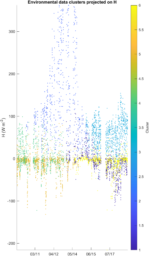
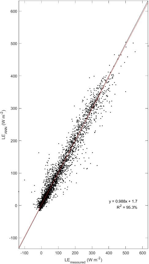
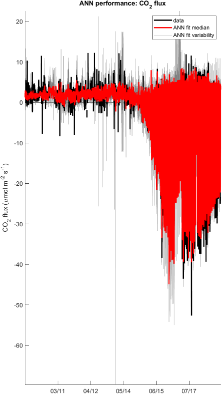
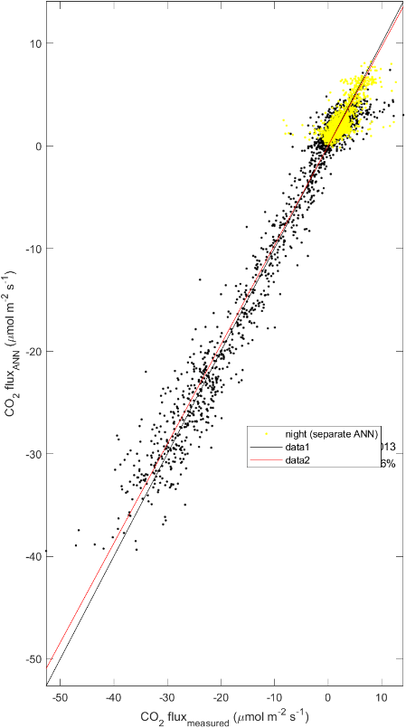
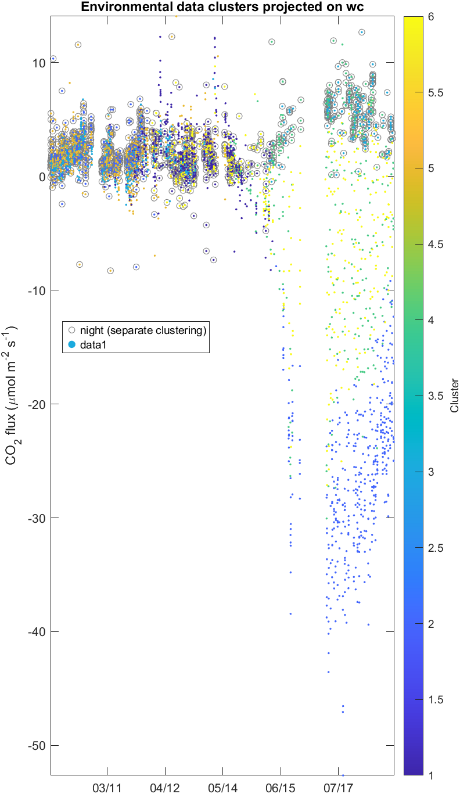
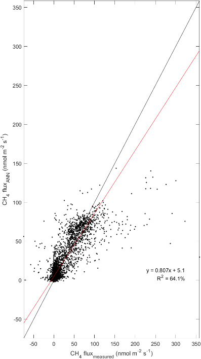
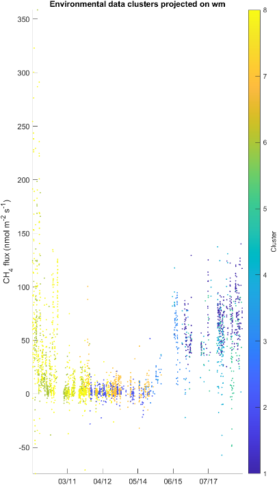
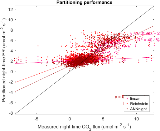
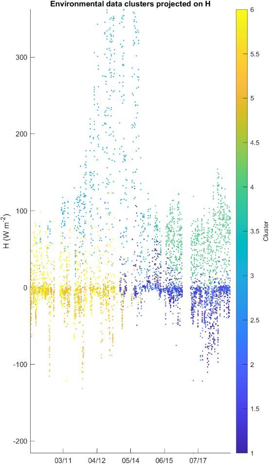
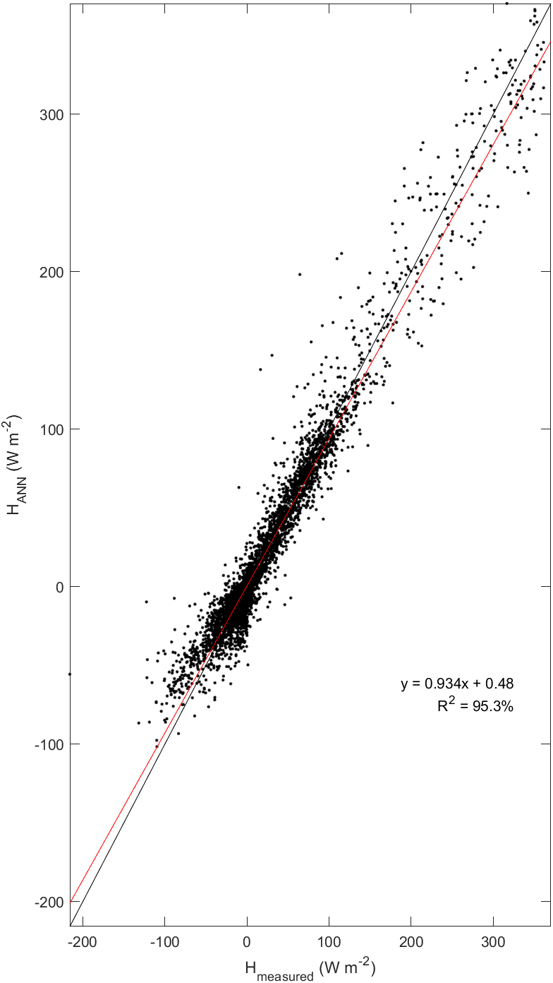
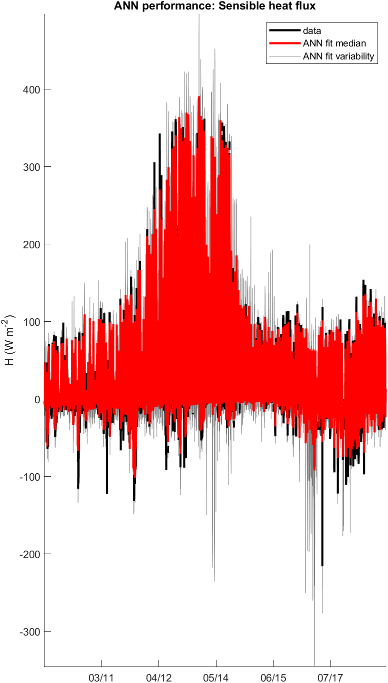
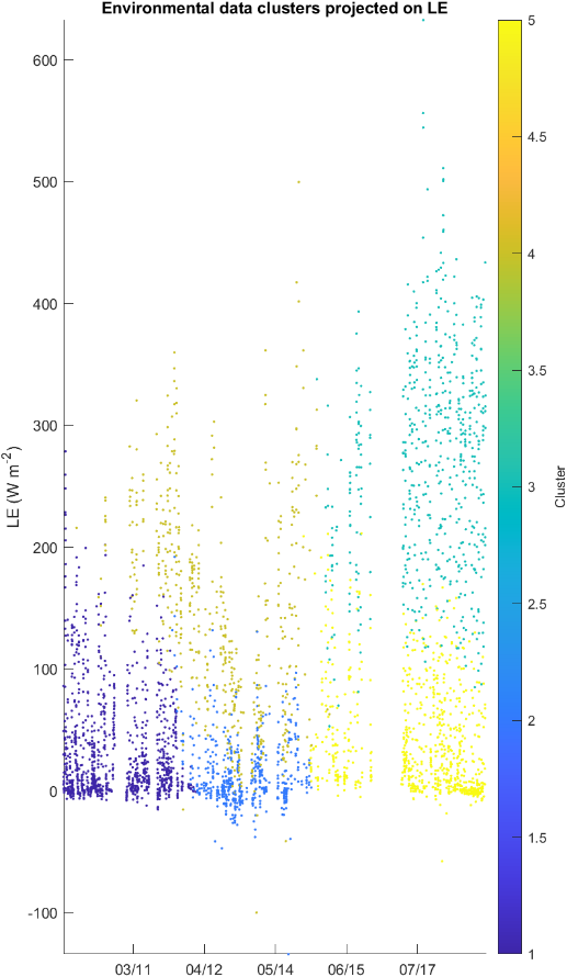
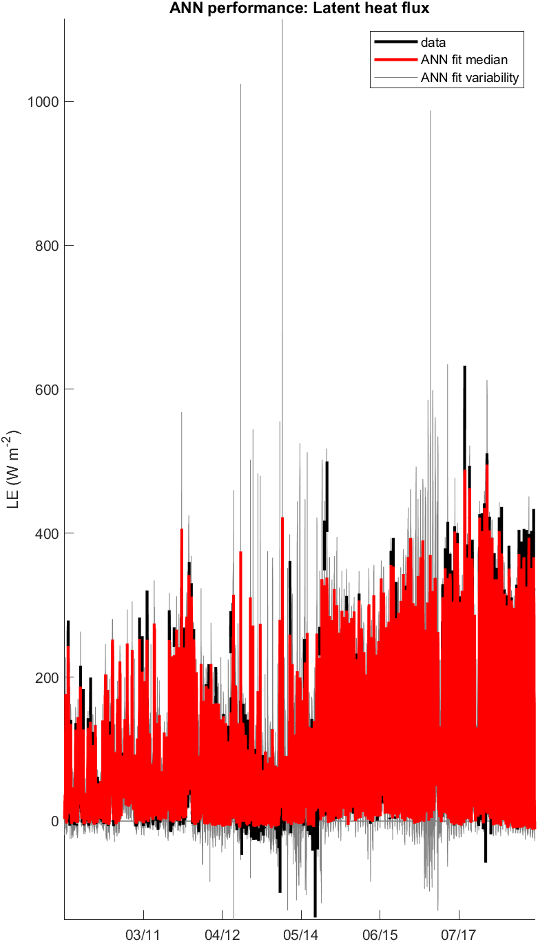
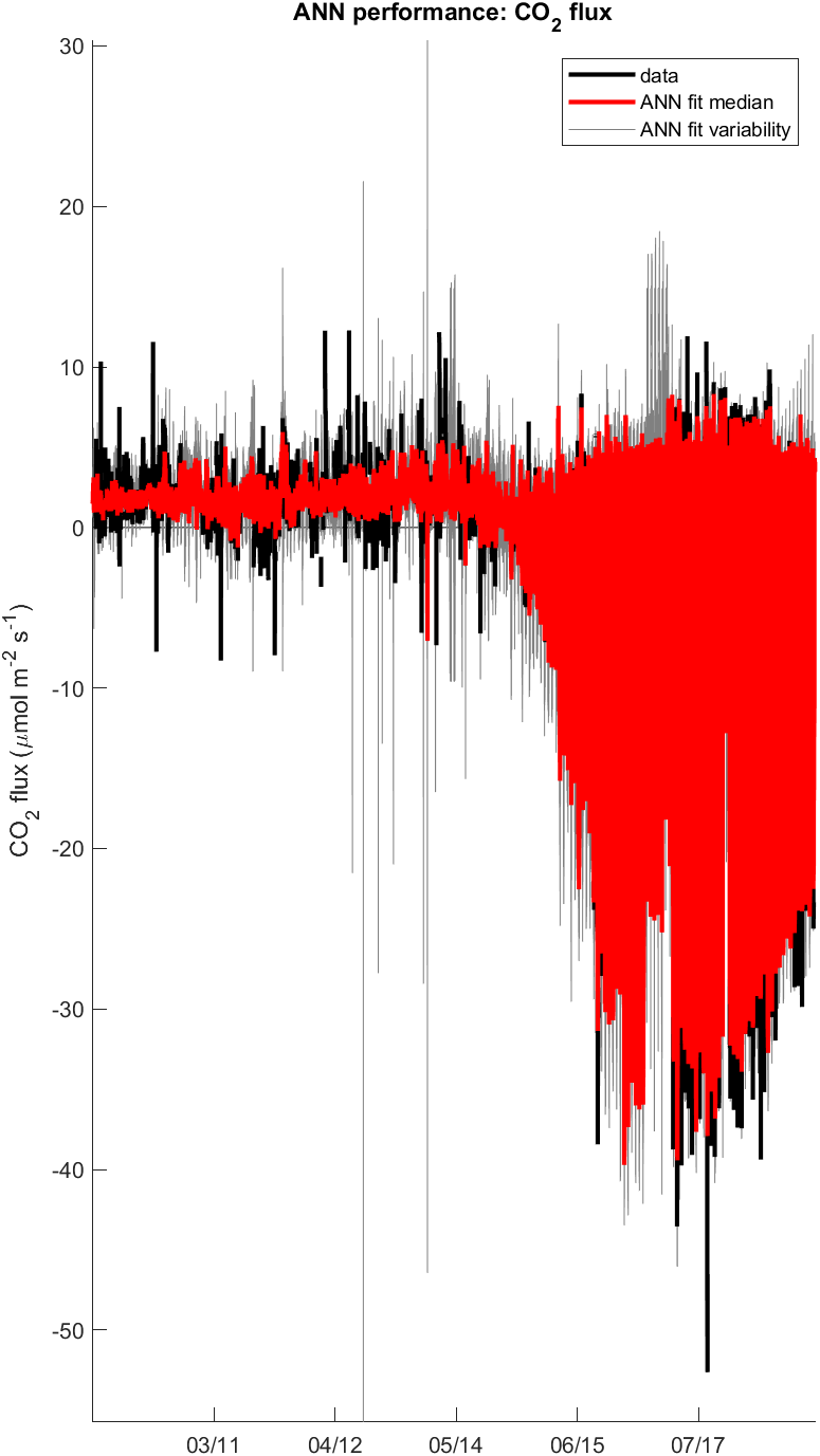
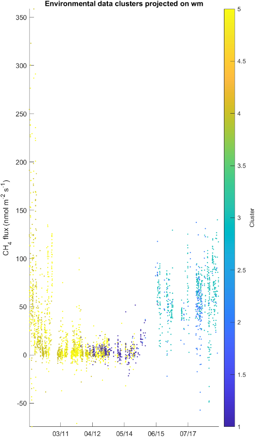
I have rerunned L3, with the Metfile input that includes Carlos Wang’s variables for Vortex. In addition, I have changed the cluster numbers and I have chosen a slightly different variables for the filling, after having discussed it with Ariane:

 

Wt: Rg, ze, az, TA_32cm, VPD, WD

Wq: TA, Rg, ze, VPD, ustar, Tsoil_2

Wc: PAR, TA, VPD, az, ustar (in the future-> decday_since_mow)

Wc GPP/ER partitioning: TA, ustar, par

Wm: WD, TA, rlong_in, vpd, ustar, LE (that it is ngf)

 

Once I rerun, the results are as follows (they are slightly better):

 

 

 

 

Total d’emissions de CO2, 7 de febrer – 21 de maig (quan van inundar el camp i la vegetació va començar a tenir presència): 17.51 mol m^-2 // 210.16 gC m^-2

Total d’emissions de CO2, 22 de maig – 16 d’agost: –40.02 mol m^-2 // -480.23 gC m^-2

Total d’emissions de CH4, 7 de febrer – 21 de Maig: 0.11 mol m^-2 // 1.37 gC m⁻²

Total d’emissions de CH4, 22 de maig – 16 d’agost:: 0.327984 mol m^-2 // 3.94 gC m^-2